%%
clear all
% Sample latitude and longitude data
ilat = 25*rand(1,50)+25;
ilon = 50*rand(1,50)-120;
% Sample data for color-coding the points
data = 10*rand(1,50);
close all
latlim=[min(ilat) ,max(ilat)];
lonlim=[min(ilon) , max(ilon)];
% find number of stations lat lon and number of data
h1 = figure(1);
ax = worldmap(latlim, lonlim);
states = shaperead('usastatehi','UseGeoCoords', true, 'BoundingBox', [lonlim', latlim']);
geoshow(ax, states, 'Facecolor', [1 1 0.9]);
hold on
map = colormap;
colorvector = map(1:64,:);
pmvect = linspace(0, max(data), 64);
for jj = 1:length(data)
%jj
colorb = interp1(pmvect, colorvector, data(jj));
plotm(ilat(jj),ilon(jj), data(jj),'o', 'MarkerEdgeColor','k','MarkerFaceColor', colorb, 'MarkerSize', 5);
hold on
end
caxis([0 max(data)])
colorbar
hold off
set(gcf,'Color','white')
Showing posts with label map. Show all posts
Showing posts with label map. Show all posts
Tuesday, March 21, 2023
Map with Latitudes and Longitudes, filled with shades
Fun maps...
Friday, December 23, 2022
Plot netcdf data on map
Plot netcdf data on map
close all clear all iwantFile ='ECMWF_utci_20201201_v1.1_con.nc' iT = double(ncread(iwantFile, 'utci')); iT2 = iT(:,:,20); iLon = double(ncread(iwantFile, 'lon')); iLat = double(ncread(iwantFile, 'lat')); load coastlines figure(1); imagesc('xdata', iLon, 'ydata', iLat , 'cdata', (iT2')); line(coastlon, coastlat, 'color', 'k') colorbar grid on; box on caxis auto set(gcf,'Color','white') xlim([-180 180]) ylim([-90 90])
Friday, July 21, 2017
Plot USA m_maps
(cc).
close all
load coastlines
states = shaperead('usastatehi',...
'UseGeoCoords', true, 'BoundingBox', [lonlim', latlim']);
figure
m_proj('miller','long',[-125 -67],'lat',[25 49.5]);
% m_gshhs_i('color','b');
% m_grid('box','fancy','tickdir','in');
m_coord('geographic'); % Switch to assuming geographic
% m_coast('patch',[1 1 0.99],'edgecolor','b');
m_coast('patch',[.98 0.98 .98],'edgecolor','none');
m_grid('box','fancy','linestyle','none','backcolor',[.8 .96 1]);
m_text(-121,38.08, '*' ,'color','r','fontweight','bold','fontsize',24); % Tahoe
m_text(-116.8,33.03, '*' ,'color','r','fontweight','bold','fontsize',24); % salton Sea
m_text( -77.8729,40.2547, '*' ,'color','r','fontweight','bold','fontsize',24); % PSU
m_text( -89.9729,33.9, '*' ,'color','r','fontweight','bold','fontsize',24); % GWN
m_text(-97.62,43.3, '*' ,'color','r','fontweight','bold','fontsize',24); % SXF
m_text(-89.37,40., '*' ,'color','r','fontweight','bold','fontsize',24); % BND
for kk = 1:length(states)
m_line(states(kk).Lon,states(kk).Lat,'linewi',0.5,'color',[200 200 200]./255);
end
set(gcf,'Color','White')
export_fig([ saveDir, 'USA_validationPoints'],'-png','-r250')
Thursday, May 26, 2016
Set Lat Lon Limits at the edge of the map
It looks nicer when you have the numbers at the edge.
setm(gca,'fontsize', 12,'PLabelLocation',[ylim(1)+0.001, mean(ylim), ylim(2)],'PLineLocation',[ylim(1)+0.001, mean(ylim), ylim(2)],...
'PLabelRound',-3,'MLabelLocation',[xlim(1), mean(xlim), xlim(2)],'MLineLocation',[xlim(1), mean(xlim), xlim(2)], 'MLabelRound',-3, ...
'Grid','on')
Thursday, April 21, 2016
M_Map Examples for matlab mapping
There are so many projections to choose from:
% Stereographic
% Orthographic
% Azimuthal Equal-area
% Azimuthal Equidistant
% Gnomonic
% Satellite
% Albers Equal-Area Conic
% Lambert Conformal Conic
% Mercator
% Miller Cylindrical
% Equidistant Cylindrical
% Oblique Mercator
% Transverse Mercator
% Sinusoidal
% Gall-Peters
% Hammer-Aitoff
% Mollweide
% Robinson
% UTM
Which one to choose?
Here are some of my favs:
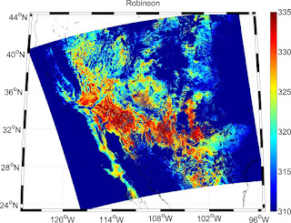
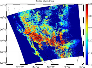
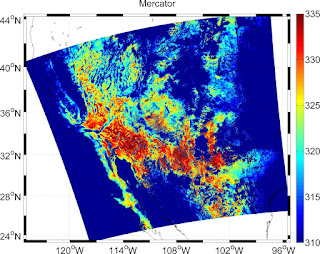
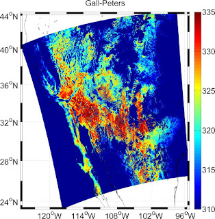
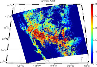
Native: examples
https://www.eoas.ubc.ca/~rich/map.html
% Stereographic
% Orthographic
% Azimuthal Equal-area
% Azimuthal Equidistant
% Gnomonic
% Satellite
% Albers Equal-Area Conic
% Lambert Conformal Conic
% Mercator
% Miller Cylindrical
% Equidistant Cylindrical
% Oblique Mercator
% Transverse Mercator
% Sinusoidal
% Gall-Peters
% Hammer-Aitoff
% Mollweide
% Robinson
% UTM
Which one to choose?
Let me quote: "Well, it depends really on how large an area you are mapping. Usually, maps of the whole world are Mercator, although often the Miller Cylindrical projection looks better because it doesn't emphasize the polar areas as much. Another choice is the Hammer-Aitoff or Mollweide (which has meridians curving together near the poles). Both are equal-area. It's probably not a good idea to use these projections for maps that don't have the equator somewhere near the middle. The Robinson projection is not equal-area or conformal, but was the choice of National Geographic (for a while, anyway), and also appears in the IPCC reports.If you are plotting something with a large north/south extent, but not very wide (say, North and South America, or the North and South Atlantic), then the Sinusoidal or Mollweide projections will look pretty good. Another choice is the Transverse Mercator, although that is usually used only for very large-scale maps.https://www.eoas.ubc.ca/~rich/private/mapug.html#p2.5
For smaller areas within one hemisphere or other (say, Australia, the United States, the Mediterranean, the North Atlantic) you might pick a conic projection. The differences between the two available conic projections are subtle, and if you don't know much about projections it probably won't make much difference which one you use.
If you get smaller than that, it doesn't matter a whole lot which projection you use. One projection I find useful in many cases is the Oblique Mercator, since you can align it along a long (but narrow) coastal area. If map limits along lines of longitude/latitude are OK, use a Transverse Mercator or Conic Projection. The UTM projection is also useful.
Polar areas are traditionally mapped using a Stereographic projection, since for some reason it looks nice to have a "bullseye" pattern of latitude lines."
Here are some of my favs:
Some examples of the projected MODIS LST data
latlim=[ (min(min(Lat11))), (max(max(Lat11)))];
lonlim=[ (min(min(Lon11))), (max(max(Lon11)))];figure(1)
% m_proj('UTM','long',lonlim,'lat',latlim);
% m_proj('Miller Cylindrical','long',lonlim,'lat',latlim);
% m_proj('Albers Equal-Area Conic','long',lonlim,'lat',latlim);
m_proj('Robinson','long',lonlim,'lat',latlim);
% m_proj('Sinusoidal','long',lonlim,'lat',latlim);
m_pcolor(Lon11,Lat11,LST11);
set(gca,'Fontsize',24)
shading interp
m_gshhs_i('color','k');
m_grid('linestyle','-.','box','fancy','tickdir','in' );
caxis([310 335])
colorbar
set(gcf,'Color','White')
title('Robinson')
set(gca,'Fontsize',24)


Native: examples
https://www.eoas.ubc.ca/~rich/map.html
Thursday, December 4, 2014
Latitude Longitude and Data on Map @matlab
I wanted to have a nice map of the global dataset given the lat/lon and the dataset.
This code is being put here so that it could be used later.
This code is being put here so that it could be used later.
boxmap = 0
% close all
latlim = [-90, 90];
lonlim = [-180, 180];
load coast
figure
if boxmap
axesm('MapProjection','lambcyln','grid','on', ...
'MapLatLimit',latlim,'MapLonLimit',lonlim,...
'MLineLocation',15, 'PLineLocation',15)
else
ax = worldmap(latlim, lonlim);
end
geoshow(lat, long,'Color', 'black' )
set(gcf,'Color','white')
for jj = 1:length(cimms)
[SunRiseSet,Day,Dec,Alt,Azm,Rad] = suncycle( latitude(jj) , longitude(jj) , [Uyear(jj) Umo(jj) Uday(jj)] , 2880 );
if SunRiseSet(2)<SunRiseSet(1)
SunRiseSet(2) = SunRiseSet(2)+24;
end
if Uhr(jj)>SunRiseSet(1) & Uhr(jj)<SunRiseSet(2)
plotm(latitude(jj),longitude(jj), jj,'o', 'MarkerEdgeColor','r','MarkerSize',8);
dayyes(jj) = 1;
else
plotm(latitude(jj),longitude(jj), jj,'o', 'MarkerEdgeColor','b','MarkerSize',8);
dayyes(jj) = 0;
end
hold on
if rem(jj,1000)==0
textm(latitude(jj),longitude(jj), sprintf('%.1d', jj), 'color', 'g')
pause(0.5)
end
end
Thursday, September 18, 2014
Map data matlab plot
Plotting Map in Matlab with the colorbar and NaNs set as transparent white.
Just call it with the lat,lon and Z (same size), and do caxis of your desire at the end. Voila!
Save it.
Just call it with the lat,lon and Z (same size), and do caxis of your desire at the end. Voila!
Save it.
function hhf = mapme(Latitude, Longitude, Z)
hhf = figure
load coast
latlim=[floor(min(min(Latitude))),ceil(max(max(Latitude)))];
lonlim=[floor(min(min(Longitude))),ceil(max(max(Longitude)))];
ax = worldmap(latlim, lonlim);
pcolorm(Latitude, Longitude, Z);
geoshow(lat, long,'Color', 'black' )
colormap;
set(gcf,'Color','white')
% map2 = colormap; map2( 64, : ) = 1; colormap(map2);
colorbar
Wednesday, September 10, 2014
Map/ Figure with white color bar assignment to the lowest value
Sometimes we need the figures or plots showing the maps. The oceans/missing values are indicated in the data as NaN or -9999. This code will plot the data with the lowest value being shown as white color.
A = rand(55);
figure;
imagesc(A)
colormap(jet(33))
map2 = colormap; map2( 1, : ) = 1; colormap(map2)
cmap = colormap; % cmap nicely puts colormap into 3 col data
colorbar
Friday, June 13, 2014
Map with inset
So, I had to zoom into NYC area with the counts of data shown for lat/lon points
here is a figure:
here is a figure:
 |
| NYC Zoomed in to show more details |
close all
latlim = [40, 45];
lonlim = [-80,-72];
% latlim = [40, 42];
% lonlim = [-80,-73];
% find number of stations lat lon and number of data
h1 = figure(1);
ax = worldmap(latlim, lonlim);
states = shaperead('usastatehi','UseGeoCoords', true, 'BoundingBox', [lonlim', latlim']);
geoshow(ax, states, 'Facecolor', [1 1 0.9]);
hold on
map = colormap;
colorvector = map(1:64,:);
pmvect = linspace(0, max(saveI), 64);
for jj = 1:41
jj
% textm(st_lat(jj),st_lon(jj), num2str(jj));
colorb = interp1(pmvect, colorvector, saveI(jj));
% plotm(Lat1(jj),Lon1(jj), jj,'o', 'MarkerEdgeColor','k','MarkerSize',saveI(jj)+1);
plotm(Lat1(jj),Lon1(jj), saveI(jj),'o', 'MarkerEdgeColor','k','MarkerFaceColor', colorb, 'MarkerSize', 5);
hold on
% textm(Lat1(jj),Lon1(jj),sprintf('%.1d', jj))
end
caxis([0 max(saveI)])
% colorbar
title('The number of Episodic (PM2.5>35\mug/m^{-3}) events in NY')
hold off
h2 = figure(2);
latlim = [40.5, 40.9];
lonlim = [-74.3,-73.5];
ax = worldmap(latlim, lonlim);
set(ax, 'FontSize', 1)
states = shaperead('usastatehi','UseGeoCoords', true, 'BoundingBox', [lonlim', latlim']);
geoshow(ax, states, 'Facecolor', [1 1 0.9]);
hold on
map = colormap;
colorvector = map(1:64,:);
pmvect = linspace(0, max(saveI), 64);
for jj = 1:41
jj
% textm(st_lat(jj),st_lon(jj), num2str(jj));
colorb = interp1(pmvect, colorvector, saveI(jj));
% plotm(Lat1(jj),Lon1(jj), jj,'o', 'MarkerEdgeColor','k','MarkerSize',saveI(jj)+1);
plotm(Lat1(jj),Lon1(jj), saveI(jj),'o', 'MarkerEdgeColor','k','MarkerFaceColor', colorb, 'MarkerSize', 5);
hold on
% textm(Lat1(jj),Lon1(jj),sprintf('%.1d', jj))
end
caxis([0 max(saveI)])
% set(findobj(gcf, 'type','axes'), 'Visible','off')
hold off
% trying to inset the figure
inset_size=0.4;
inset_size=inset_size*.7;
figure;
new_fig=gcf;
main_fig = findobj(h1,'Type','axes');
h_main = copyobj(main_fig,new_fig);
set(h_main,'Position',get(main_fig,'Position'))
colorbar
inset_fig = findobj(h2,'Type','axes');
h_inset = copyobj(inset_fig,new_fig);
ax=get(main_fig,'Position');
% set(h_inset,'Position', [.7*ax(1)+ax(3)-inset_size .5*ax(2)+ax(4)-inset_size inset_size inset_size])
set(h_inset,'Position', [0.3*ax(1) 1.5*ax(2) inset_size*2 inset_size])
Tuesday, May 13, 2014
Northeast region map
Basic code in matlab to create northeast states.
latlim = [ 35 48];
lonlim = [-85 -65];
% want states
ilatlim = [ 37 46];
ilonlim = [-80 -69];
figure
ax = usamap(latlim,lonlim);
axis off
% axesm('MapProjection','conic')
% The Lambert Conformal Conic Projection is often used for maps of the conterminous United States.
% Here is the map projection usamap selected:
% getm(gca,'MapProjection')
% ans =
% lambert
% Next, use shaperead to read U.S. state polygon boundaries from the usastatehi shapefile into a geostruct named states:
states = shaperead('usastatehi',...
'UseGeoCoords', true, 'BoundingBox', [ilonlim', ilatlim']);
% Make a symbolspec to create a political map using the polcmap function:
faceColors = makesymbolspec('Polygon',...
{'INDEX', [1 numel(states)], ...
'FaceColor', polcmap(numel(states))});
% Display the filled polygons with geoshow:
geoshow(ax, states, 'SymbolSpec', faceColors)
% Extract the names for states within the window from the geostruct and use textm to plot them at the label points provided by the geostruct:
for k = 1:numel(states)
labelPointIsWithinLimits =...
37 < states(k).LabelLat &&...
latlim(2) > states(k).LabelLat &&...
-82.5 < states(k).LabelLon &&...
lonlim(2) > states(k).LabelLon;
if labelPointIsWithinLimits
textm(states(k).LabelLat,...
states(k).LabelLon, states(k).Name, ...
'HorizontalAlignment', 'center', 'FontSize', 15)
end
end
tightmap
Thursday, May 8, 2014
Creating DINEOF movie for AOD 2006-2008
Basic code for getting movie for the tabfilled variable
load('box_Lat_lon.mat');
for kk = 1:length(tabfilled)
%For plots
latlim =([35 46]);
lonlim =([-85 -69]);
% fig_title = sprintf('MODIS AOD %i-%i-%i',file_mm,file_dd,file_yy);
h1 = figure(1)
% orient landscape;
ax = worldmap(latlim, lonlim);
states = shaperead('usastatehi','UseGeoCoords', true, 'BoundingBox', [lonlim', latlim']);
geoshow(ax, states, 'FaceColor', [1 1 1]);
surfacem(box_lat,box_lon,tabfilled(:,:,kk));
h1=gca;
set(h1,'CLimMode','Manual','CLim',[0, 1]);
h2=colorbar('vert','FontSize',12);
title(['2008 Day: ', num2str(kk)],'FontSize',14);
M(kk) = getframe(h1);
end
% Output the movie as an avi file
movie2avi(M,'AOD_IDWMovie2008r1.avi', 'compression','None', 'fps',2);
Saturday, February 1, 2014
Plot the spatial grid on map in matlab
We will need the latgrid and longitude grid with equal size to that of the variable, say newT
figure
latlim = [37,45 ]; lonlim = [-82 ,-70];
ax = worldmap(latlim, lonlim);
states = shaperead('usastatehi','UseGeoCoords', true, 'BoundingBox', [lonlim', latlim']);
geoshow(ax, states, 'Facecolor', [1 1 0.9]);
surfacem(latgrid,longrid,newT);
Subscribe to:
Posts (Atom)


