Insert degree symbol in MS word

Note to self:

1. Press and hold "Ctrl"
2. Press and hold "Shift"
3. Press "@"
4. Release "Ctrl", "Shift"
5. Press "Space Bar"

installing #altair #python #conda

>conda install altair --channel conda-forge

The following packages will be downloaded:

    package                    |            build
    ---------------------------|-----------------
    conda-4.1.8                |           py35_0         247 KB
    pandas-0.18.1              |      np110py35_0         6.9 MB  conda-forge
    vega-0.4.1                 |           py35_1         904 KB  conda-forge
    altair-1.0.0               |           py35_0         1.6 MB  conda-forge
    ------------------------------------------------------------
                                           Total:         9.6 MB
Linking packages ...
[vega                ]|#########################                         |  50%
C:\Users\Userme>"C:\Users\Userme\AppData\Local\Continuum\Anaconda3\Scripts\jupyter-nbextension.exe" install vega --py --sys-prefix   && if errorlevel 1 exit 1

Just for my note

    To initialize this nbextension in the browser every time the notebook (or other app) loads:

          jupyter nbextension enable vega --py --sys-prefix

The documentation:
https://github.com/ellisonbg/altair

Create Clickable imagesc for 2D data

Looking at the figure is fun, specially if you can click and get the values. So, created this little function which can give you title and data tips @cursor location.

function imagesca(x, titlewant)
h = figure;
imagesc(x);
colorbar
try
    title(titlewant);
catch ME
    title('Figure')
end
datacursormode on

Print a large poster on multiple A4/paper

There are two ways:
1. Save the (powerpoint) document as  pdf.
2. Open the pdf, print.
3. Select the appropriate options in the poster option in the page size and handling section
4. The options are Tile scale: 200% for example, overlap by few tenth of the inches
5. Cutmarks and labels etc are optional #4 does the magic!

Another way that I learned from the internet is to paste the picture in the excel sheet. The excel is smart enough to segment the pic into multiple pages. And, I used to think that extra flowing line being printed into second page was a bad feature in excel! :)

Dropbox over server

Well, I had some failures in the past. So, I wanted to try again.
First, I had to run headless install via command line.
Then ran the Dropbox daemon from the newly created .dropbox-dist folder.
~/.dropbox-dist/dropboxd
That got me a unique link to link dropbox account to cloud.
Then I got the dropbox.py code from the help page (https://www.dropbox.com/install?os=lnx)

Rest was not bad!

Here are some of the commands that I had to run... because I wanted to exclude bunch of folders from syncing. I wish there was "include" option instead of "exclude".

~/bin/dropbox.py exclude add ~/Dropbox/MyExclude1 ~/Dropbox/MyExclude2 

~/bin/dropbox.py exclude list 

~/bin/dropbox.py help ~/bin/dropbox.py status ~/bin/dropbox.py start

Plot LST

Just a code to plot LST

Lat  = double(hdfread(filewant,  'Latitude' ));
Lon  =  double(hdfread(filewant,  'Longitude' ));
LST = 0.02* double(hdfread(filewant,  'LST' ));
LST(LST==0)=NaN;
figure

load coast
latlim=[floor(min(min(Lat))),ceil(max(max(Lat))) ]; lonlim=[floor(min(min(Lon))),ceil(max(max(Lon))) ];
ax = worldmap(latlim, lonlim);
surfacem(Lat, Lon, LST);
geoshow(lat, long,'Color', 'black' )
colormap; set(gcf,'Color','white')
map2 = colormap; map2( 1, : ) = 0; colormap(map2);
colorbar % saveas(gcf, 'plotHDF.png', 'png') close all
caxis([ 290 330])

Chrome: Add keyboard shortcut to your favorite website

This trick works on Google chrome. 

• Right click on the address bar
• Edit Search Engines
• Scroll to the bottom of the list
• Give the name, keyword (eg. gs: for google scholar), then URL.

You can put %s in place of query.

Matlab Colorbar: LST

I think I found a good one! (Sorry intensity, no one prints grayscale pics these days... they just read on-screen).

r1 = [1 0];
g1 = [0 0];
b1 =  [1 1];
rgb1 = [r1; g1; b1]';
rgba = interp1([1 2],rgb1, linspace(1,2,16 ));
r1 = [0 0];
g1 = [0 1];
b1 =  [1 1];
rgb1 = [r1; g1; b1]';
rgbb = interp1([1 2],rgb1, linspace(1,2,11 ));

r1 = [0 0];
g1 = [1 1];
b1 =  [1 0];
rgb1 = [r1; g1; b1]';
rgbc = interp1([1 2],rgb1, linspace(1,2,10));

r1 = [0 1];
g1 = [1 1];
b1 =  [0 0];
rgb1 = [r1; g1; b1]';
rgbd = interp1([1 2],rgb1, linspace(1,2,11 ));

r1 = [ 1 1];
g1 = [1 0];
b1 =  [0 0];
rgb2 = [r1; g1; b1]';
rgbe= interp1([1 2],rgb2, linspace(1,2,16));

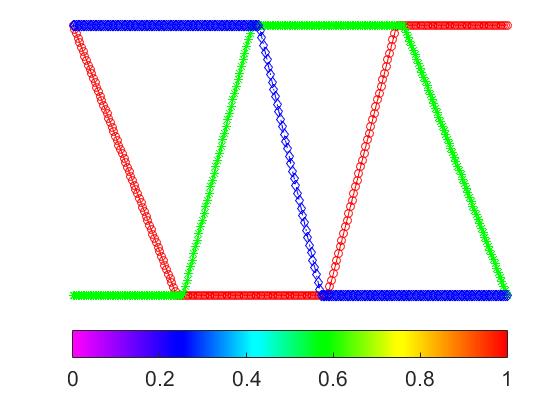
newNDVI = [rgba;rgbb;rgbc;rgbd;rgbe];

newNDVI= interp1( newNDVI, linspace(1,64,256));


%
figure
plot([1:256],newNDVI(:,1), 'ro-'); hold on
plot([1:256],newNDVI(:,2), 'g*-');
plot([1:256],newNDVI(:,3), 'bd-.');
xlim([1 256])

colormap(newNDVI );
cmap = colormap; % cmap nicely puts colormap into 3 col data
% colorbar
caxis([0 1])
hc = colorbar('southoutside');
set(hc, 'FontSize', 16)

 axis off; set(gcf,'Color','White')

I can append white and or black at the end for distinction, if needed.

Insert the date and time into the google docs

This first appeared here ... http://ajabgajab.blogspot.com/2015/01/insert-date-and-time-into-google-docs.html 

This is how you insert the date and time to the google docs

1. Go to the Google document/new document.
2. Go to the Tools/Script Editor, and insert the following script at the bottom of the scripts.
This will create a new menu. You can modify the code to change the appearance of the month/date.
3. See the end note to add automated date entry!

The code is available below/ at pastebin.
http://pastebin.com/QFpTRQ3h

function onOpen() {
  var ui = DocumentApp.getUi();
  // Or FormApp or SpreadsheetApp.
  ui.createMenu('Insert Date')
      .addItem('Insert Date', 'insertDate')
      .addToUi();

}

function insertDate() {
  var cursor = DocumentApp.getActiveDocument().getCursor();
  if (cursor) {
      // Attempt to insert text at the cursor position. If insertion returns null,
      // then the cursor's containing element doesn't allow text insertions.
      var d = new Date();
      var dd = d.getDate();
      var hrs = d.getHours();
      var min = d.getMinutes();
      dd = pad(dd, 2)
      var mm = d.getMonth() + 1; //Months are zero based
      mm = pad(mm, 2)
      var yyyy = d.getFullYear();
    var date =  "Date: "+mm + "-" +dd + "-" + yyyy+ "::"+hrs+":"+min +"\n";
      var element = cursor.insertText(date);
      if (element) {
        element.setBold(true);
      } else {
        DocumentApp.getUi().alert('Cannot insert text at this cursor location.');
      }
    } else {
      DocumentApp.getUi().alert('Cannot find a cursor in the document.');
  }

}
function pad (str, max) {
  str = str.toString();
  return str.length < max ? pad("0" + str, max) : str;
}

--- 
--> 

Note:
If you add the following function call inside the onOpen() function:
  insertDate();
Then you will get automated insertion of date and time. Great for logging the daily notes!!!

function onOpen() {
  var ui = DocumentApp.getUi();
  // Or FormApp or SpreadsheetApp.
  ui.createMenu('Insert Date')
      .addItem('Insert Date', 'insertDate')
      .addToUi();

  insertDate();

}

Colormap for NDVI

Setting up NDVI colorbar can be tricky! You want a nice representation of the vegetation and bare surfaces in the map.

1. I found an easy way would be to flip the default matlab summer color bar upside down!
colormap('summer')
map2 = (colormap);
map2 = flipud(map2);
colormap(map2);
cmap = colormap;
It looks like:

However, the negatives are not treated nicely. For the first approximation, I could set x<0 == 0.

2. Found a nice one:
https://publiclab.org/notes/cfastie/08-26-2014/new-ndvi-colormap
The colorbar is nice, but, I was not much happy with the squeezed RBG dance!

3. Having seen them, I wanted to create my own.
I combined the inverted summer with the graded b/w scheme.  The idea is to set inverted summer for x > 0 with  the gray image for x < 0!
So, I wrote this small piece!

r1 = [0 1];
g1 = [0 1];
b1 =  [0 1];
rgb1 = [r1; g1; b1]';
rgbt = interp1([1 2],rgb1, linspace(1,2,32 ));

r1 = [ 1 0];
g1 = [1 0.5];
b1 =  [0.4 0.4];
rgb2 = [r1; g1; b1]';
rgbb= interp1([1 2],rgb2, linspace(1,2,32 ));

newNDVI = [rgbt;rgbb];

figure
colormap(newNDVI );
cmap = colormap; % cmap nicely puts colormap into 3 col data
% colorbar
caxis([-1 1])
hc = colorbar('southoutside');
set(hc, 'FontSize', 16)

 axis off; set(gcf,'Color','White')

You can set that linspace limit to 128, and make 256x3 colormap, making a smooth colorbar.
The new NDVI colorbar looks like:

The color scheme looks like:

For the first half, it goes from dark to bright, and then smoothly to green from yellow at the center!

Try it! and let me know if you like this scheme for NDVI!
Here is a small preview. I changed the lower rgbb matrix to 224x3 arrays which nicely set yellow limit at ~0.2! (some info on NDVI for the cusious minds: http://earthobservatory.nasa.gov/Features/MeasuringVegetation/measuring_vegetation_2.php)

Forcing Matlab colorbar to display climits

Matlab sometimes can not register the upper and lower limits of the color bar when the figures are saved (eg with export_fig). 

I found a way around it:

instead of setting caxis limit at the exact values, increase/decrease the upper/lower limit

caxis([0.94 0.99] )

to >> caxis([0.94 0.99001] )

This worked for me!

Set Lat Lon Limits at the edge of the map

It looks nicer when you have the numbers at the edge.

setm(gca,'fontsize', 12,'PLabelLocation',[ylim(1)+0.001, mean(ylim), ylim(2)],'PLineLocation',[ylim(1)+0.001, mean(ylim), ylim(2)],...
    'PLabelRound',-3,'MLabelLocation',[xlim(1), mean(xlim), xlim(2)],'MLineLocation',[xlim(1), mean(xlim), xlim(2)], 'MLabelRound',-3, ...
     'Grid','on')

Colormap Stark #matlab colorbar

I wanted to have a colormap which had a great degree of contrast, and was not really a rainbow scheme.

I have tried to solve this issue by poking at different colormaps
http://usefulcodes.blogspot.com/2015/06/colormap-hotjet.html
(very close, but keeps the rainbow defect flat intensity for the large part in the middle.)
http://usefulcodes.blogspot.com/2015/06/colormap-goofy-matlab.html
(looks green and goofy! Did not like it.)
http://usefulcodes.blogspot.com/2015/06/matlab-colormap-rose.html
(has nice monotonic intensity gradient, but not that beautiful on maps.)
See the examples: http://usefulcodes.blogspot.com/search/label/colormap
I present you a new one! Colormap "stark".
This does have the defect of not linearly increasing the intensity, but does not stay flat in the middle. It has two saddles, allowing the left/right contrast. I like it so far.
Well, it is inspired from the LST image from MODIS
http://neo.sci.gsfc.nasa.gov/view.php?datasetId=MOD11C1_M_LSTDA

175	256	255
100	249	255
50	223	253
10	191	252
9	144	252
12	106	255
11	79	254
26	56	254
34	38	255
50	34	255
79	33	255
85	33	255
101	34	255
132	35	255
150	36	255
177	39	255
217	36	255
243	35	255
255	35	213
255	34	175
255	30	143
255	36	110
255	34	88
255	33	65
255	44	35
255	72	35
254	95	39
255	116	45
254	138	41
254	160	46
255	183	45
255	199	46
255	210	47
253	225	47
254	230	75
256	256	110
R	G	B

newN = 1:64;

isn = floor(linspace(1,64,36));
%RGB = [R G B];
R1 = RGB(:,1);
G1 = RGB(:,2);
B1 = RGB(:,3);

Rn = runmean(interp1(isn, R1, newN),2);
Gn = runmean(interp1(isn, G1, newN),2);
Bn = runmean(interp1(isn, B1, newN),2);

newC=  [Rn', Gn', Bn']./256;


close all
figure ;
plot(newN, Rn, 'r-')
hold on
plot(newN, Gn, 'G-')
plot(newN, Bn, 'b-')
colormap(newC);
colorbar('southoutside')
ylim([0 260])
xlim([1 64])
legend('R', 'G', 'B','Location','southoutside','Orientation','horizontal')
xlabel('C-index')
ylabel('R,G,B')
export_fig([ 'RGB-colormap'   ],'-jpeg','-r250')

figure;
plot(newN, sum(newC,2)./3, 'r-')
ylabel('Intensity')
xlabel('C-index')
xlim([1 64])
export_fig([ 'RGB-intensity' ],'-jpeg','-r250')

Here is an alternate

175	256	255
100	249	255
50	223	253
10	191	252
9	144	252
12	106	255
11	79	254
26	56	254
34	38	255
50	25	255
79	15	255
85	15	255
101	30	255
132	50	255
150	70	255
177	80	255
217	100	255
243	100	255
255	80	213
255	70	175
255	50	143
255	30	110
255	15	88
255	25	65
255	44	35
255	72	35
254	95	39
255	116	45
254	138	41
254	160	46
255	183	45
255	199	46
255	225	47
253	240	47
254	250	75
256	256	129
R	G	B

It adds whiteness in the middle, creating W shaped swing to the green pallets.

M_Map Examples for matlab mapping

There are so many projections to choose from:
%      Stereographic
%      Orthographic
%      Azimuthal Equal-area
%      Azimuthal Equidistant
%      Gnomonic
%      Satellite
%      Albers Equal-Area Conic
%      Lambert Conformal Conic
%      Mercator
%      Miller Cylindrical
%      Equidistant Cylindrical
%      Oblique Mercator
%      Transverse Mercator
%      Sinusoidal
%      Gall-Peters
%      Hammer-Aitoff
%      Mollweide
%      Robinson
%      UTM
Which one to choose?

Let me quote: "Well, it depends really on how large an area you are mapping. Usually, maps of the whole world are Mercator, although often the Miller Cylindrical projection looks better because it doesn't emphasize the polar areas as much. Another choice is the Hammer-Aitoff or Mollweide (which has meridians curving together near the poles). Both are equal-area. It's probably not a good idea to use these projections for maps that don't have the equator somewhere near the middle. The Robinson projection is not equal-area or conformal, but was the choice of National Geographic (for a while, anyway), and also appears in the IPCC reports.If you are plotting something with a large north/south extent, but not very wide (say, North and South America, or the North and South Atlantic), then the Sinusoidal or Mollweide projections will look pretty good. Another choice is the Transverse Mercator, although that is usually used only for very large-scale maps.
For smaller areas within one hemisphere or other (say, Australia, the United States, the Mediterranean, the North Atlantic) you might pick a conic projection. The differences between the two available conic projections are subtle, and if you don't know much about projections it probably won't make much difference which one you use.
If you get smaller than that, it doesn't matter a whole lot which projection you use. One projection I find useful in many cases is the Oblique Mercator, since you can align it along a long (but narrow) coastal area. If map limits along lines of longitude/latitude are OK, use a Transverse Mercator or Conic Projection. The UTM projection is also useful.
Polar areas are traditionally mapped using a Stereographic projection, since for some reason it looks nice to have a "bullseye" pattern of latitude lines."

https://www.eoas.ubc.ca/~rich/private/mapug.html#p2.5

Here are some of my favs:

latlim=[ (min(min(Lat11))), (max(max(Lat11)))];
lonlim=[ (min(min(Lon11))), (max(max(Lon11)))];figure(1)
% m_proj('UTM','long',lonlim,'lat',latlim);
% m_proj('Miller Cylindrical','long',lonlim,'lat',latlim);
% m_proj('Albers Equal-Area Conic','long',lonlim,'lat',latlim);
m_proj('Robinson','long',lonlim,'lat',latlim);
% m_proj('Sinusoidal','long',lonlim,'lat',latlim);

m_pcolor(Lon11,Lat11,LST11);
set(gca,'Fontsize',24)
shading interp
m_gshhs_i('color','k');
m_grid('linestyle','-.','box','fancy','tickdir','in' );
caxis([310 335])
colorbar
set(gcf,'Color','White')
title('Robinson')
set(gca,'Fontsize',24)

Some examples of the projected MODIS LST data



Native: examples
https://www.eoas.ubc.ca/~rich/map.html

Matlab Plot Latitude and Longitude with degree symbol on the axis label

Not the complete code, but it does the job.

close all
load coast
cfigure( 40, 20);
plot(long, lat, 'k')
grid on
% s = sprintf('45%c', char(176));

set(gca,'XLim',[-180 180])
set(gca,'YLim',[-180/2 180/2])
set(gca,'XTick',[-180:40: 180])
set(gca,'YTick',[-90:30: 90])

xt=get(gca,'xtick');
for k=1:numel(xt);
xt1{k}=sprintf('%d°',xt(k));
end
set(gca,'xticklabel',xt1);

xt=get(gca,'ytick');
for k=1:numel(xt);
xt1{k}=sprintf('%d°',xt(k));
end
set(gca,'yticklabel',xt1);

set(gca,'Fontsize',26)

annotation('textbox', [.15  .232 0.16  0.1 ],'EdgeColor',[ 0 0 0] )

% xlim([-180 180])
% ylim([-90 90])
hold on
plot(longitude(dayyes==0), latitude(dayyes==0), 'o', 'MarkerEdgeColor','b','MarkerSize',5);
plot(longitude(dayyes==1),latitude(dayyes==1), '*', 'MarkerEdgeColor','r','MarkerSize',6);
text(-167,-50,  sprintf('* Day Profile  ' ), 'color', 'r', 'FontSize', 26)
text(-167,-60,  sprintf('o Night Profile' ), 'color', 'b', 'FontSize', 26)
%    annotation('textbox', [-175  -55 20  15 ],'EdgeColor',[0 0 0] )
ylabel('Latitude ', 'FontSize', 26)
xlabel('Longitude ', 'FontSize', 26)
set(gcf,'Color','white')

Readability Statistics in owrd

readability features in the word count are interesting one to pass at.

In Word 2013/2010, File>Option>Proofing
In word 2007, search for proofing option

Then under spelling and grammar section of the display menu, check the "Show readability statistics".
This will enable readability statistics.

A usual rule of thumb is that  the Flesch-Kincaid Grade (FKG) Level  should be around 10-12, and the Flesch Reading Ease should be between 60-70.
The FKG level is between 1-12, and represents how many years of US school is needed to understand the document.
There is also passive sentence score. While technical documents may be written with some passive statements, business documents are written with active sentences.

Find the abbreviations in word

To Find the abbreviations in the document,
Go to find, advanced, more and then set search options to "Use wildcards".
Find the following:

<[A-Z]{2,}>

Do find a reading highlight, and then highlight all.

Minus sign is another issue

Symbol			Unicode
hyphen minus sign N-dash M-dash	– − – —	f-f f−f f–f f—f	002D or 2010 2212 2013 2014

Plotyy equivalent of Bar and scatter plots

It was not so easy to replace the plotyy code with the following:
The idea is simple: plot bars, hold on and then plot scatter.
The problems were axes limits and labels not alignting properly.

% Create figure
close all
figure1 = cfigure(30,10);

% Create axes
axes1 = axes('Parent',figure1, 'YTick',[0 1 2 3]);%,...

 xlim(axes1,[min(dvec_d) max(dvec_d)]);

%  Uncomment the following line to preserve the Y-limits of the axes
ylim(axes1,[0 3]);
box(axes1,'on');
hold(axes1,'on');

% Create ylabel
ylabel('PWV (cm)','FontSize',14);


% Create axes
axes2 = axes('Parent',figure1,'HitTest','off','Color','none',...
   'YTick',[0.94 0.96 0.98 1],...
    'YAxisLocation','right', 'XTick',linspace(min(dvec_d) , max(dvec_d) , 24));
 xlim(axes2,[min(dvec_d) max(dvec_d)]);
 ylim(axes2,[0.94 1]);
hold(axes2,'on');

% Create ylabel
ylabel('MOD21 \epsilon_{29}','FontSize',14);

% Create bar
 bar(dvec_d,pwv_d5,'FaceColor',[0.8 0.8 0.5],'EdgeColor',[0.5 0.99 0.9],'Parent',axes1);
 %set(axes1, 'ydir', 'reverse'); % this will put hanging bars


set(axes1,'xtick',[])
set(axes1,'xticklabel',[])
hold on
% Create scatter
scatter(dvec_d,mod21_e295d, 'Parent',axes2,'MarkerEdgeColor',[1 0 0],'Marker','*');
set(axes2,'xtick',[])
set(axes2,'xticklabel',[])
set(axes2,'xticklabel',[])

%         datetick('x','yyyy-mm' );.
datetick('x','yyyy-mm', 'keeplimits')
title(' PWV and Emissivity Time Series','FontSize',14); % add a title and define the font size
xlabel('Time ( 2003-2005)')
hold on
line( dvec_d, 1.5* ones(length(dvec_d)), 'Parent', axes1  )

set(axes2,{'ycolor'},{'r' })  
    

States Line disappearing in map: Solved

In matlab you can extract the states lat/lon information and plot them so that the problem of states lines disappearing can be solved.
here is an example where you can extract the state lat/lon data from the axis limit boundary and make lats/lons variables. These can be plotted with geoshow.

figure(1)
latlim = [35 45];
lonlim = [-115 -100];
    ax = worldmap(latlim, lonlim);

  states = shaperead('usastatehi','UseGeoCoords', true, 'BoundingBox', [lonlim', latlim']);
   geoshow(ax, states, 'FaceColor', [1 1 1], 'LineWidth', 3);
   lats = [];
lons = [];
for aa = 1:length(states)
lats = horzcat(lats, states(aa).Lat);
lons = horzcat(lons, states(aa).Lon);
end
geoshow(lats,lons,'DisplayType','Line', 'Color', [0 1 0])
% latlim=[floor(min(min(SatLat))),ceil(max(max(SatLat)))];
% lonlim=[floor(min(min(SatLon))),ceil(max(max(SatLon)))];
surfacem(SatLat, SatLon, double(c66in5));
hold on
plotm( y,x ) % polygon

plotm(37 , -105 , 1, 'yo')
set(gcf,'Color','white')

Latex Installed on Windows 10

MiKTeX installed the Latex.exe in the following location:
Not so obvious, Is it?

C:\Users\myusername\AppData\Local\Programs\MiKTeX 2.9\miktex\bin\x64

Insert Landscape pages in paper

We are often faced with a long table in the middle of the document. I used to insert a text box, then ratate it so that final view had a rotated table. However, when I went on to edit the table/text box content, it would rotate back... and things are not so easy!

This solution is easier than what I used to do:
Simply highlight the text/table to be rotated into the landscape, then go to margin, select custom, then do landscape page orientation for the selection. Voila! I am assuming that the table will occupy the whole page.

The following is from Office Support page:
https://support.office.com/en-us/article/Rotate-page-orientation-between-portrait-and-landscape-in-Word-2010-14952283-8BA7-4A52-82B9-A8487A5674B4

Use portrait and landscape orientation in the same document

1. Select the pages or paragraphs that you want to change to portrait or landscape orientation.
   NOTE    If you select some but not all of the text on a page to change to portrait or landscape orientation, Word places the selected text on its own page, and the surrounding text on separate pages.
2. On the Page Layout tab, in the Page Setup group, click Margins.
   
3. Click Custom Margins.
4. On the Margins tab, click Portrait or Landscape.
5. In the Apply to list, click Selected text..

Matlab Map plot with limits

It is not so obvious to plot matlab maps with latitude and longitude limits on the axes' ends.
The following code helped me.

figure
ax = worldmap(ylim, xlim);
states = shaperead('usastatehi','UseGeoCoords', true, 'BoundingBox', [xlim', ylim']);
geoshow(ax, states, 'FaceColor', [1 1 1]);
surfacem(LatLsatf1, LonLsatf1,NDVI1);
colormap('summer')
title(['NDVI (', DOY, ')'], 'FontSize', 20)
map2 = (colormap);
map2 = flipud(map2);
colormap(map2);
cmap = colormap; % cmap nicely puts colormap into 3 col data
% colorbar
caxis([-0  1])

setm(gca,'fontsize', 12,'PLabelLocation',[ylim(1), mean(ylim), ylim(2)],'PLineLocation',[ylim(1), mean(ylim), ylim(2)],...
    'PLabelRound',-3,'MLabelLocation',[xlim(1), mean(xlim), xlim(2)],'MLineLocation',[xlim(1), mean(xlim), xlim(2)], 'MLabelRound',-3, ...
     'Grid','on')