Map with Latitudes and Longitudes, filled with shades

Fun maps...

 

%%

clear all

 

% Sample latitude and longitude data

ilat = 25*rand(1,50)+25;

ilon = 50*rand(1,50)-120;

% Sample data for color-coding the points

data = 10*rand(1,50);

 

close all

latlim=[min(ilat) ,max(ilat)];

lonlim=[min(ilon) , max(ilon)];

% find number of stations lat lon and number of data

h1 = figure(1);

ax = worldmap(latlim, lonlim);

states = shaperead('usastatehi','UseGeoCoords', true, 'BoundingBox', [lonlim', latlim']);

geoshow(ax, states, 'Facecolor', [1 1 0.9]);

hold on

map = colormap;

colorvector = map(1:64,:);

pmvect = linspace(0, max(data), 64);

for jj = 1:length(data)

    %jj

colorb = interp1(pmvect, colorvector, data(jj));

plotm(ilat(jj),ilon(jj), data(jj),'o', 'MarkerEdgeColor','k','MarkerFaceColor', colorb, 'MarkerSize', 5);

hold on   

end

caxis([0  max(data)])

colorbar

hold off

set(gcf,'Color','white')

Plot netcdf data on map

Plot netcdf data on map

close all clear all iwantFile ='ECMWF_utci_20201201_v1.1_con.nc' iT = double(ncread(iwantFile, 'utci')); iT2 = iT(:,:,20); iLon = double(ncread(iwantFile, 'lon')); iLat = double(ncread(iwantFile, 'lat')); load coastlines figure(1); imagesc('xdata', iLon, 'ydata', iLat , 'cdata', (iT2')); line(coastlon, coastlat, 'color', 'k') colorbar grid on; box on caxis auto set(gcf,'Color','white') xlim([-180 180]) ylim([-90 90])

Combine PDFs in mac terminal

Combine PDF

gs -q -dNOPAUSE -dBATCH -sDEVICE=pdfwrite -sOutputFile=BindCoverAll.pdf Cover1.pdf Editorial_Cover_TOC.pdf JNPS732021_Combined.pdf

Plotting NPP hdf data

A sample code to plot the NPP data

The data source:

http://orca.science.oregonstate.edu/1080.by.2160.monthly.hdf.vgpm.m.chl.m.sst.php 

 filewant = 'cafe.2007001.hdf';

 

info = hdfinfo(filewant);

 

% This is how you can investigate the file structure...

info.SDS

%% note the names

info.SDS.Attributes.Name

%% note the values of the attributes

info.SDS.Attributes.Value

%% read the npp variable

npp  = double(hdfread(filewant,  'npp' ));

 

npp(npp==-9999) = NaN;

% figure;

% imagesc(npp)

npp = flipud(npp); % because npp is flipped upside down wrt lat/lon for map

 

%%

iLat = linspace(-90,90,1080);

iLon = linspace(-180,180,2160);

[Lat, Lon] = ndgrid(iLat,iLon);

 

figure

load coastlines % coastineData.mat

latlim=[floor(min(min(Lat))),ceil(max(max(Lat))) ]; 

lonlim=[floor(min(min(Lon))),ceil(max(max(Lon))) ];

ax = worldmap(latlim, lonlim);

surfacem(Lat, Lon, npp);

geoshow(coastlat, coastlon,'Color', 'k' )

colormap; set(gcf,'Color','white')

colormap jet

map2 = colormap; 

map2( 1, : ) = 1; colormap(map2);

colorbar 

 

title('global dataset')

  

 

disp('Next we will try to crop out the area of interest')

%% This is an example of how to crop out to the area of interest...

iLat2 = linspace(-15,45,1080);

iLon2 = linspace(-90,0,2160);

[Lat2, Lon2] = ndgrid(iLat2,iLon2);

 

F = griddedInterpolant(Lat,Lon,npp); % read doc griddedInterpolant

npp_crop = F(Lat2,Lon2);

 

%

 

figure

load coastlines % coastineData.mat

latlim=[floor(min(min(Lat2))),ceil(max(max(Lat2))) ]; 

lonlim=[floor(min(min(Lon2))),ceil(max(max(Lon2))) ];

ax = worldmap(latlim, lonlim);

surfacem(Lat2, Lon2, npp_crop);

geoshow(coastlat, coastlon,'Color', 'k' )

colormap; set(gcf,'Color','white')

colormap jet

map2 = colormap; 

map2( 1, : ) = 1; colormap(map2);

colorbar 

title('NPP (mgC m-2 day-1)')

Alternative code that I have seen:

 https://hdfeos.org/zoo/OTHER/npp_2010361_hdf.m

 

Alternating color in table conflicts with xcolor

T

My issue was trying to use the table with alternate color in a latex document with the termcal.
\usepackage[table]{xcolor}    % loads also »colortbl«

There were conflicts.

\PassOptionsToPackage{table}{xcolor} inserted before the \documentclass{..} fixed the issue!

Yes, Thanks to
https://tex.stackexchange.com/questions/5363/how-to-create-alternating-rows-in-a-table

DiskPart Recovering SD card

My problem:
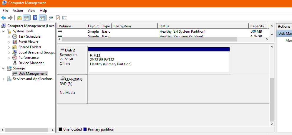
Tried installing Raspberian into 32 GB SD card. The file system went corrupt-somehow. Could not recover the other big part in windows because windows system.
The diskmanagement system showed the 30GB space in dark, which could not be accessed by simple formatting or change of the drive letter.

So, I had to go commando.
Went to the command mode.
Windows> CMD (admin mode)
Then executed the following codes...

Now I can see the whole SD card space!

diskpart

Microsoft DiskPart version 10.0.ccc

Copyright (C) 1999-2013 Microsoft Corporation.
On computer: xxx

DISKPART> list disk

  Disk ###  Status         Size     Free     Dyn  Gpt
  --------  -------------  -------  -------  ---  ---
  Disk 0    Online          476 GB      0 B        *
  Disk 1    Online          476 GB      0 B        *
  Disk 2    Online           29 GB    26 GB

DISKPART> select disk 2

Disk 2 is now the selected disk.

DISKPART> clean

DiskPart succeeded in cleaning the disk.

DISKPART> create partition primary

DiskPart succeeded in creating the specified partition.

DISKPART> (then formatted the disk)

Change Printers Default Single Sided Setting #mac

 Well, there is an easy way...

http://localhost:631/

This prompted me to do
cupsctl WebInterface=yes
to the terminal... which enabled opening up the printer options... then I could set up the duplex printing.
Went to
http://localhost:631/admin/#General
Then, I had to select "Two-sided, Long-edge binding".

This enabled printing on both sides.

Plot USA m_maps

(cc).

  close all
 load coastlines
states = shaperead('usastatehi',...
        'UseGeoCoords', true, 'BoundingBox', [lonlim', latlim']);
figure
m_proj('miller','long',[-125 -67],'lat',[25 49.5]);
% m_gshhs_i('color','b');
% m_grid('box','fancy','tickdir','in');
m_coord('geographic');           % Switch to assuming geographic
% m_coast('patch',[1 1 0.99],'edgecolor','b');
  m_coast('patch',[.98 0.98 .98],'edgecolor','none');
    m_grid('box','fancy','linestyle','none','backcolor',[.8 .96 1]);
m_text(-121,38.08,  '*' ,'color','r','fontweight','bold','fontsize',24); % Tahoe
m_text(-116.8,33.03,  '*' ,'color','r','fontweight','bold','fontsize',24); % salton Sea

m_text( -77.8729,40.2547,  '*' ,'color','r','fontweight','bold','fontsize',24); % PSU
m_text( -89.9729,33.9,  '*' ,'color','r','fontweight','bold','fontsize',24); % GWN
m_text(-97.62,43.3,  '*' ,'color','r','fontweight','bold','fontsize',24); % SXF
m_text(-89.37,40.,  '*' ,'color','r','fontweight','bold','fontsize',24); % BND

for kk = 1:length(states)
m_line(states(kk).Lon,states(kk).Lat,'linewi',0.5,'color',[200 200 200]./255);
end
set(gcf,'Color','White')

export_fig([ saveDir,  'USA_validationPoints'],'-png','-r250')

From Google Fusion table to Google Earth Engine!

First I made a Google Fusion table with few points with Latitue and Logitude geo-coded Names.
Then imported into fusion table

// import the fusion table
var Da = ee.FeatureCollection('ft:18RyzwhfBU0TVFa4HWFEp778Tkd9YV-X1pE_Q1hq6').geometry();

// Set center of map
Map.centerObject(Da, 6);

// show the layer
Map.addLayer(Da);

The cryptic code in the FeatureCollection is the ID of the fusion table.

See an example here
https://code.earthengine.google.com/78e9375af2c31dbb5381dede4a46d922

Insert degree symbol in MS word

Note to self:

1. Press and hold "Ctrl"
2. Press and hold "Shift"
3. Press "@"
4. Release "Ctrl", "Shift"
5. Press "Space Bar"

installing #altair #python #conda

>conda install altair --channel conda-forge

The following packages will be downloaded:

    package                    |            build
    ---------------------------|-----------------
    conda-4.1.8                |           py35_0         247 KB
    pandas-0.18.1              |      np110py35_0         6.9 MB  conda-forge
    vega-0.4.1                 |           py35_1         904 KB  conda-forge
    altair-1.0.0               |           py35_0         1.6 MB  conda-forge
    ------------------------------------------------------------
                                           Total:         9.6 MB
Linking packages ...
[vega                ]|#########################                         |  50%
C:\Users\Userme>"C:\Users\Userme\AppData\Local\Continuum\Anaconda3\Scripts\jupyter-nbextension.exe" install vega --py --sys-prefix   && if errorlevel 1 exit 1

Just for my note

    To initialize this nbextension in the browser every time the notebook (or other app) loads:

          jupyter nbextension enable vega --py --sys-prefix

The documentation:
https://github.com/ellisonbg/altair

Create Clickable imagesc for 2D data

Looking at the figure is fun, specially if you can click and get the values. So, created this little function which can give you title and data tips @cursor location.

function imagesca(x, titlewant)
h = figure;
imagesc(x);
colorbar
try
    title(titlewant);
catch ME
    title('Figure')
end
datacursormode on

Print a large poster on multiple A4/paper

There are two ways:
1. Save the (powerpoint) document as  pdf.
2. Open the pdf, print.
3. Select the appropriate options in the poster option in the page size and handling section
4. The options are Tile scale: 200% for example, overlap by few tenth of the inches
5. Cutmarks and labels etc are optional #4 does the magic!

Another way that I learned from the internet is to paste the picture in the excel sheet. The excel is smart enough to segment the pic into multiple pages. And, I used to think that extra flowing line being printed into second page was a bad feature in excel! :)

Dropbox over server

Well, I had some failures in the past. So, I wanted to try again.
First, I had to run headless install via command line.
Then ran the Dropbox daemon from the newly created .dropbox-dist folder.
~/.dropbox-dist/dropboxd
That got me a unique link to link dropbox account to cloud.
Then I got the dropbox.py code from the help page (https://www.dropbox.com/install?os=lnx)

Rest was not bad!

Here are some of the commands that I had to run... because I wanted to exclude bunch of folders from syncing. I wish there was "include" option instead of "exclude".

~/bin/dropbox.py exclude add ~/Dropbox/MyExclude1 ~/Dropbox/MyExclude2 

~/bin/dropbox.py exclude list 

~/bin/dropbox.py help ~/bin/dropbox.py status ~/bin/dropbox.py start

Plot LST

Just a code to plot LST

Lat  = double(hdfread(filewant,  'Latitude' ));
Lon  =  double(hdfread(filewant,  'Longitude' ));
LST = 0.02* double(hdfread(filewant,  'LST' ));
LST(LST==0)=NaN;
figure

load coast
latlim=[floor(min(min(Lat))),ceil(max(max(Lat))) ]; lonlim=[floor(min(min(Lon))),ceil(max(max(Lon))) ];
ax = worldmap(latlim, lonlim);
surfacem(Lat, Lon, LST);
geoshow(lat, long,'Color', 'black' )
colormap; set(gcf,'Color','white')
map2 = colormap; map2( 1, : ) = 0; colormap(map2);
colorbar % saveas(gcf, 'plotHDF.png', 'png') close all
caxis([ 290 330])

Chrome: Add keyboard shortcut to your favorite website

This trick works on Google chrome. 

• Right click on the address bar
• Edit Search Engines
• Scroll to the bottom of the list
• Give the name, keyword (eg. gs: for google scholar), then URL.

You can put %s in place of query.

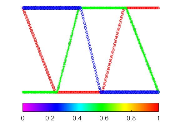
Matlab Colorbar: LST

I think I found a good one! (Sorry intensity, no one prints grayscale pics these days... they just read on-screen).

r1 = [1 0];
g1 = [0 0];
b1 =  [1 1];
rgb1 = [r1; g1; b1]';
rgba = interp1([1 2],rgb1, linspace(1,2,16 ));
r1 = [0 0];
g1 = [0 1];
b1 =  [1 1];
rgb1 = [r1; g1; b1]';
rgbb = interp1([1 2],rgb1, linspace(1,2,11 ));

r1 = [0 0];
g1 = [1 1];
b1 =  [1 0];
rgb1 = [r1; g1; b1]';
rgbc = interp1([1 2],rgb1, linspace(1,2,10));

r1 = [0 1];
g1 = [1 1];
b1 =  [0 0];
rgb1 = [r1; g1; b1]';
rgbd = interp1([1 2],rgb1, linspace(1,2,11 ));

r1 = [ 1 1];
g1 = [1 0];
b1 =  [0 0];
rgb2 = [r1; g1; b1]';
rgbe= interp1([1 2],rgb2, linspace(1,2,16));

newNDVI = [rgba;rgbb;rgbc;rgbd;rgbe];

newNDVI= interp1( newNDVI, linspace(1,64,256));


%
figure
plot([1:256],newNDVI(:,1), 'ro-'); hold on
plot([1:256],newNDVI(:,2), 'g*-');
plot([1:256],newNDVI(:,3), 'bd-.');
xlim([1 256])

colormap(newNDVI );
cmap = colormap; % cmap nicely puts colormap into 3 col data
% colorbar
caxis([0 1])
hc = colorbar('southoutside');
set(hc, 'FontSize', 16)

 axis off; set(gcf,'Color','White')

I can append white and or black at the end for distinction, if needed.

Insert the date and time into the google docs

This first appeared here ... http://ajabgajab.blogspot.com/2015/01/insert-date-and-time-into-google-docs.html 

This is how you insert the date and time to the google docs

1. Go to the Google document/new document.
2. Go to the Tools/Script Editor, and insert the following script at the bottom of the scripts.
This will create a new menu. You can modify the code to change the appearance of the month/date.
3. See the end note to add automated date entry!

The code is available below/ at pastebin.
http://pastebin.com/QFpTRQ3h

function onOpen() {
  var ui = DocumentApp.getUi();
  // Or FormApp or SpreadsheetApp.
  ui.createMenu('Insert Date')
      .addItem('Insert Date', 'insertDate')
      .addToUi();

}

function insertDate() {
  var cursor = DocumentApp.getActiveDocument().getCursor();
  if (cursor) {
      // Attempt to insert text at the cursor position. If insertion returns null,
      // then the cursor's containing element doesn't allow text insertions.
      var d = new Date();
      var dd = d.getDate();
      var hrs = d.getHours();
      var min = d.getMinutes();
      dd = pad(dd, 2)
      var mm = d.getMonth() + 1; //Months are zero based
      mm = pad(mm, 2)
      var yyyy = d.getFullYear();
    var date =  "Date: "+mm + "-" +dd + "-" + yyyy+ "::"+hrs+":"+min +"\n";
      var element = cursor.insertText(date);
      if (element) {
        element.setBold(true);
      } else {
        DocumentApp.getUi().alert('Cannot insert text at this cursor location.');
      }
    } else {
      DocumentApp.getUi().alert('Cannot find a cursor in the document.');
  }

}
function pad (str, max) {
  str = str.toString();
  return str.length < max ? pad("0" + str, max) : str;
}

--- 
--> 

Note:
If you add the following function call inside the onOpen() function:
  insertDate();
Then you will get automated insertion of date and time. Great for logging the daily notes!!!

function onOpen() {
  var ui = DocumentApp.getUi();
  // Or FormApp or SpreadsheetApp.
  ui.createMenu('Insert Date')
      .addItem('Insert Date', 'insertDate')
      .addToUi();

  insertDate();

}

Colormap for NDVI

Setting up NDVI colorbar can be tricky! You want a nice representation of the vegetation and bare surfaces in the map.

1. I found an easy way would be to flip the default matlab summer color bar upside down!
colormap('summer')
map2 = (colormap);
map2 = flipud(map2);
colormap(map2);
cmap = colormap;
It looks like:

However, the negatives are not treated nicely. For the first approximation, I could set x<0 == 0.

2. Found a nice one:
https://publiclab.org/notes/cfastie/08-26-2014/new-ndvi-colormap
The colorbar is nice, but, I was not much happy with the squeezed RBG dance!

3. Having seen them, I wanted to create my own.
I combined the inverted summer with the graded b/w scheme.  The idea is to set inverted summer for x > 0 with  the gray image for x < 0!
So, I wrote this small piece!

r1 = [0 1];
g1 = [0 1];
b1 =  [0 1];
rgb1 = [r1; g1; b1]';
rgbt = interp1([1 2],rgb1, linspace(1,2,32 ));

r1 = [ 1 0];
g1 = [1 0.5];
b1 =  [0.4 0.4];
rgb2 = [r1; g1; b1]';
rgbb= interp1([1 2],rgb2, linspace(1,2,32 ));

newNDVI = [rgbt;rgbb];

figure
colormap(newNDVI );
cmap = colormap; % cmap nicely puts colormap into 3 col data
% colorbar
caxis([-1 1])
hc = colorbar('southoutside');
set(hc, 'FontSize', 16)

 axis off; set(gcf,'Color','White')

You can set that linspace limit to 128, and make 256x3 colormap, making a smooth colorbar.
The new NDVI colorbar looks like:

The color scheme looks like:

For the first half, it goes from dark to bright, and then smoothly to green from yellow at the center!

Try it! and let me know if you like this scheme for NDVI!
Here is a small preview. I changed the lower rgbb matrix to 224x3 arrays which nicely set yellow limit at ~0.2! (some info on NDVI for the cusious minds: http://earthobservatory.nasa.gov/Features/MeasuringVegetation/measuring_vegetation_2.php)

Forcing Matlab colorbar to display climits

Matlab sometimes can not register the upper and lower limits of the color bar when the figures are saved (eg with export_fig). 

I found a way around it:

instead of setting caxis limit at the exact values, increase/decrease the upper/lower limit

caxis([0.94 0.99] )

to >> caxis([0.94 0.99001] )

This worked for me!