There are so many projections to choose from:
% Stereographic
% Orthographic
% Azimuthal Equal-area
% Azimuthal Equidistant
% Gnomonic
% Satellite
% Albers Equal-Area Conic
% Lambert Conformal Conic
% Mercator
% Miller Cylindrical
% Equidistant Cylindrical
% Oblique Mercator
% Transverse Mercator
% Sinusoidal
% Gall-Peters
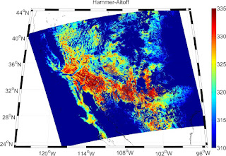
% Hammer-Aitoff
% Mollweide
% Robinson
% UTM
Which one to choose?
Here are some of my favs:
Native: examples
https://www.eoas.ubc.ca/~rich/map.html
% Stereographic
% Orthographic
% Azimuthal Equal-area
% Azimuthal Equidistant
% Gnomonic
% Satellite
% Albers Equal-Area Conic
% Lambert Conformal Conic
% Mercator
% Miller Cylindrical
% Equidistant Cylindrical
% Oblique Mercator
% Transverse Mercator
% Sinusoidal
% Gall-Peters
% Hammer-Aitoff
% Mollweide
% Robinson
% UTM
Which one to choose?
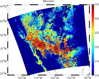
Let me quote: "Well, it depends really on how large an area you are mapping. Usually, maps of the whole world are Mercator, although often the Miller Cylindrical projection looks better because it doesn't emphasize the polar areas as much. Another choice is the Hammer-Aitoff or Mollweide (which has meridians curving together near the poles). Both are equal-area. It's probably not a good idea to use these projections for maps that don't have the equator somewhere near the middle. The Robinson projection is not equal-area or conformal, but was the choice of National Geographic (for a while, anyway), and also appears in the IPCC reports.If you are plotting something with a large north/south extent, but not very wide (say, North and South America, or the North and South Atlantic), then the Sinusoidal or Mollweide projections will look pretty good. Another choice is the Transverse Mercator, although that is usually used only for very large-scale maps.https://www.eoas.ubc.ca/~rich/private/mapug.html#p2.5
For smaller areas within one hemisphere or other (say, Australia, the United States, the Mediterranean, the North Atlantic) you might pick a conic projection. The differences between the two available conic projections are subtle, and if you don't know much about projections it probably won't make much difference which one you use.
If you get smaller than that, it doesn't matter a whole lot which projection you use. One projection I find useful in many cases is the Oblique Mercator, since you can align it along a long (but narrow) coastal area. If map limits along lines of longitude/latitude are OK, use a Transverse Mercator or Conic Projection. The UTM projection is also useful.
Polar areas are traditionally mapped using a Stereographic projection, since for some reason it looks nice to have a "bullseye" pattern of latitude lines."
Here are some of my favs:
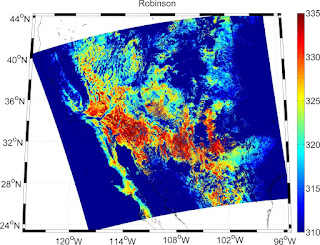
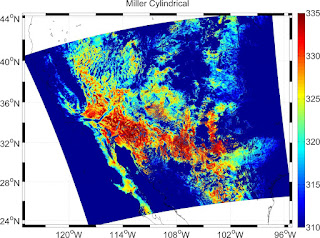
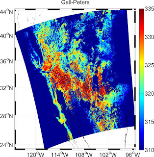
Some examples of the projected MODIS LST data
latlim=[ (min(min(Lat11))), (max(max(Lat11)))];
lonlim=[ (min(min(Lon11))), (max(max(Lon11)))];figure(1)
% m_proj('UTM','long',lonlim,'lat',latlim);
% m_proj('Miller Cylindrical','long',lonlim,'lat',latlim);
% m_proj('Albers Equal-Area Conic','long',lonlim,'lat',latlim);
m_proj('Robinson','long',lonlim,'lat',latlim);
% m_proj('Sinusoidal','long',lonlim,'lat',latlim);
m_pcolor(Lon11,Lat11,LST11);
set(gca,'Fontsize',24)
shading interp
m_gshhs_i('color','k');
m_grid('linestyle','-.','box','fancy','tickdir','in' );
caxis([310 335])
colorbar
set(gcf,'Color','White')
title('Robinson')
set(gca,'Fontsize',24)


Native: examples
https://www.eoas.ubc.ca/~rich/map.html